Currently, there are 8 functions associated with the
calculate verb in the sgsR package:
| Algorithm | Description |
|---|---|
calculate_representation() |
Determine representation of strata in existing sample unit |
calculate_distance() |
Per pixel distance to closest access
vector |
calculate_pcomp() |
Principal components of input
mraster
|
calculate_sampsize() |
Estimated sample sizes based on relative standard error |
calculate_allocation() |
Proportional / optimal / equal / manual allocation |
calculate_coobs() |
Detail how existing sample units are
distributed among mraster
|
calculate_pop() |
Population level information (PCA / quantile matrix /
covariance matrix) of mraster
|
calculate_lhsOpt() |
Determine optimal Latin hypercube sampling parameters including sample size |
calculate_representation()
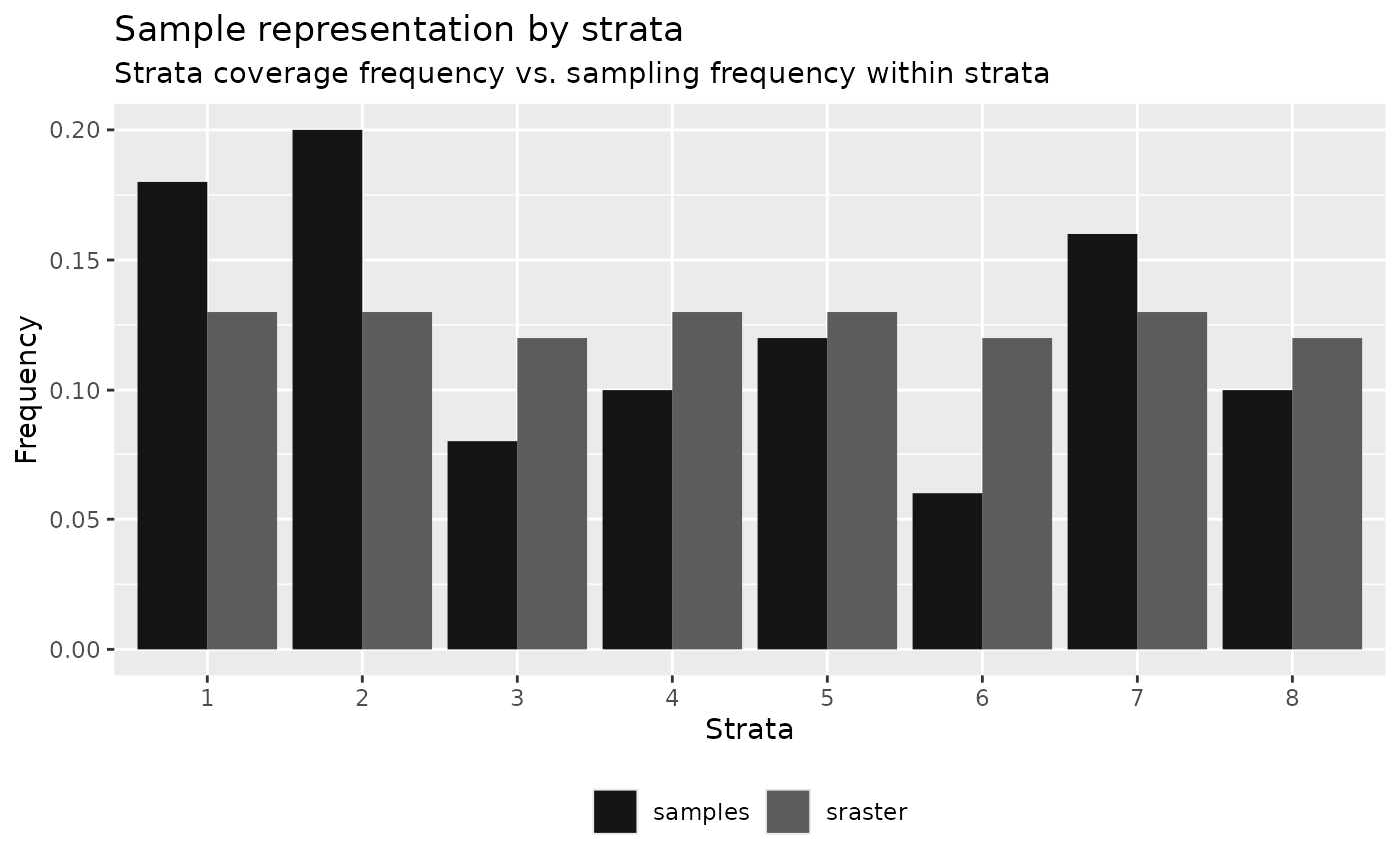
calculate_representation() function allows the users to
verify how a stratification is spatially represented in an
existing sample. Result in tabular and graphical (if
plot = TRUE) outputs that compare strata coverage frequency
and sampling frequency.
#--- quantile sraster ---#
quantiles <- strat_quantiles(
  mraster = mraster$zq90,
  nStrata = 8
)

#--- random samples ---#
srs <- sample_srs(
  raster = sraster,
  nSamp = 50
)

#--- calculate representation ---#
calculate_representation(
  sraster = quantiles,
  existing = srs,
  plot = TRUE
)
#> # A tibble: 8 × 6
#>   strata srasterFreq sampleFreq diffFreq nSamp  need
#>    <dbl>       <dbl>      <dbl>    <dbl> <int> <dbl>
#> 1      1        0.13       0.1   -0.03       5     2
#> 2      2        0.13       0.12  -0.0100     6     1
#> 3      3        0.12       0.16   0.04       8    -2
#> 4      4        0.13       0.2    0.07      10    -3
#> 5      5        0.13       0.12  -0.0100     6     1
#> 6      6        0.12       0.12   0          6     0
#> 7      7        0.13       0.14   0.0100     7     0
#> 8      8        0.12       0.04  -0.08       2     4
The tabular output presents the frequency of coverage for each strata
(srasterFreq) (what % of the landscape does the strata
cover) and the sampling frequency within each strata
(sampleFreq) (what % of total existing samples
are in the strata). The difference (diffFreq) between
coverage frequency and sampling frequency determines whether the values
are over-represented (positive numbers) or under-represented (negative
numbers). This value translates to a discrete need
attribute that defines whether there is a need to add or remove samples
to meet the number of samples necessary to be considered representative
of the spatial coverage of strata inputted in sraster.
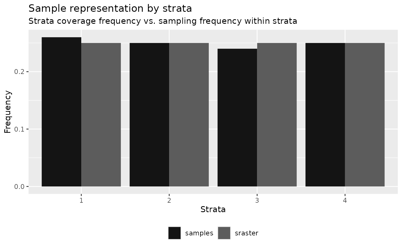
Performing the algorithm on a sample set derived using
sample_strat() exhibits proportional sampling to strata
coverage given that samples were allocated proportionally to spatial
coverage.
calculate_representation(
  sraster = sraster,
  existing = existing,
  plot = TRUE
)
#> # A tibble: 4 × 6
#>   strata srasterFreq sampleFreq diffFreq nSamp  need
#>    <dbl>       <dbl>      <dbl>    <dbl> <int> <dbl>
#> 1      1        0.25       0.26   0.0100    51    -1
#> 2      2        0.25       0.25   0         50     0
#> 3      3        0.25       0.24  -0.0100    49     1
#> 4      4        0.25       0.25   0         50     0
TIP!
Presence of very small (negligible) differences between
srasterFreq and sampleFreq is common.
In these situations, it is important for the user to determine
whether to add or remove the samples.
calculate_distance
calculate_distance() uses input raster and
access data and outputs the per pixel distance to the
nearest access point. This algorithm has a specific value for
constraining sampling protocols, such as with
sample_clhs(), where the output raster layer can be used as
the cost for the constraint. The output raster consists of
the input appended with the calculated distance layer
(dist2access). The slope parameters also
exists to calculate slope distance instead of geographic distance, which
becomes very handy in the case of steep mountainous areas and is faster
from a computational point of view. If slope == TRUE, the
mraster provided should be a digital terrain model.
calculate_distance(
  raster = sraster, # input
  access = access, # define access road network
  plot = TRUE
) # plot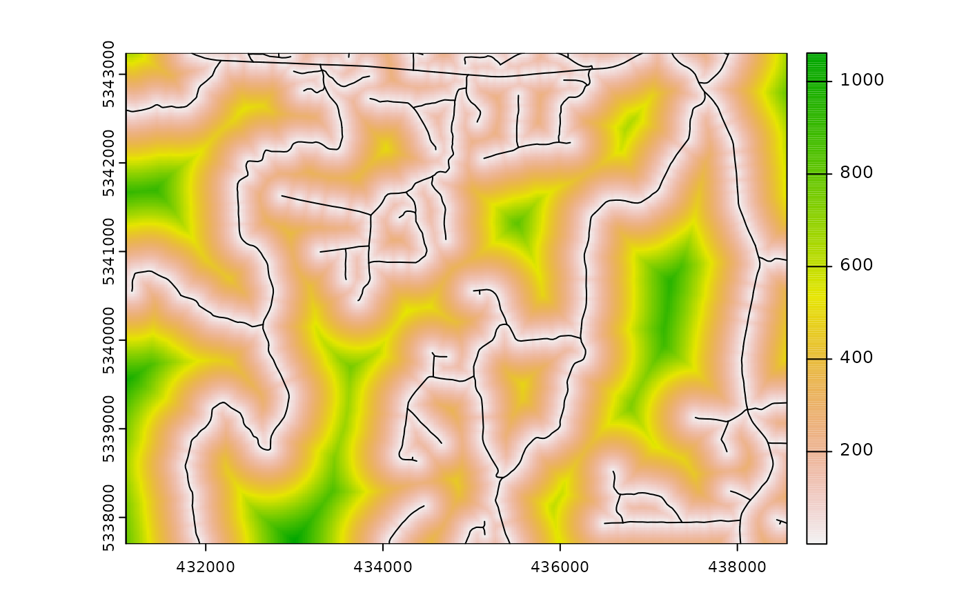
#> class       : SpatRaster
#> size        : 277, 373, 2  (nrow, ncol, nlyr)
#> resolution  : 20, 20  (x, y)
#> extent      : 431100, 438560, 5337700, 5343240  (xmin, xmax, ymin, ymax)
#> coord. ref. : UTM Zone 17, Northern Hemisphere
#> source(s)   : memory
#> varnames    : mraster
#>               mraster
#> names       : strata,  dist2access
#> min values  :      1, 6.621213e-03
#> max values  :      4, 1.061660e+03
This function performs considerably slower when
access has many features. Consider mergeing features for
improved efficiency.
calculate_pcomp
calculate_pcomp() uses mraster as the input
and performs principal component analysis. The number of components
defined by the nComp parameter specifies the number of
components that will be rasterized.
calculate_pcomp(
  mraster = mraster, # input
  nComp = 3, # number of components to output
  plot = TRUE, # plot
  details = TRUE
) # details about the principal component analysis appended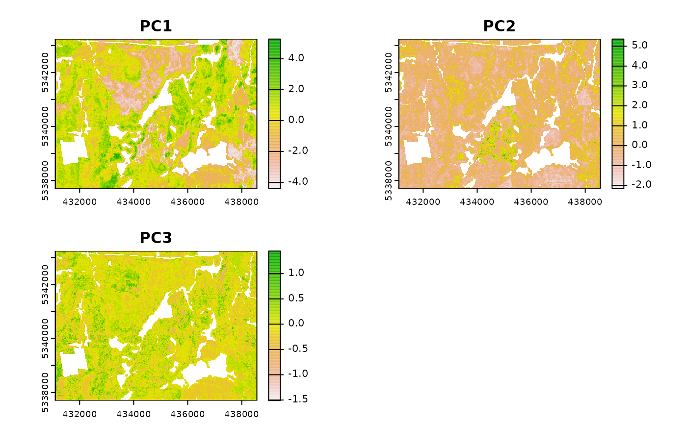
#> $pca
#> Standard deviations (1, .., p=3):
#> [1] 1.5479878 0.7359109 0.2493371
#>
#> Rotation (n x k) = (3 x 3):
#>                PC1        PC2        PC3
#> zq90     0.6286296  0.1795433  0.7566961
#> pzabove2 0.5104140 -0.8293596 -0.2272450
#> zsd      0.5867729  0.5290812 -0.6130014
#>
#> $raster
#> class       : SpatRaster
#> size        : 277, 373, 3  (nrow, ncol, nlyr)
#> resolution  : 20, 20  (x, y)
#> extent      : 431100, 438560, 5337700, 5343240  (xmin, xmax, ymin, ymax)
#> coord. ref. : UTM Zone 17, Northern Hemisphere
#> source(s)   : memory
#> varnames    : mraster
#>               mraster
#>               mraster
#> names       :       PC1,       PC2,       PC3
#> min values  : -4.402269, -2.155242, -1.510955
#> max values  :  5.282663,  5.357801,  1.446156
calculate_sampsize
calculate_sampsize() function allows the user to
estimate an appropriate sample size using the relative standard error
(rse) of input metrics. If the input mraster
contains multiple layers, the sample sizes will be determined for all
layers. If plot = TRUE and rse is defined, a
sequence of rse values will be visualized with the
indicators and the values for the matching sample size.
#--- determine sample size based on relative standard error (rse) of 1% ---#
calculate_sampsize(
  mraster = mraster,
  rse = 0.01
)
#>   nSamp  rse      var
#> 1  1394 0.01     zq90
#> 2  1341 0.01 pzabove2
#> 3  1859 0.01      zsd
#--- change default threshold sequence values ---#
#--- if increment and rse are not divisible the closest value will be taken ---#
p <- calculate_sampsize(
  mraster = mraster,
  rse = 0.025,
  start = 0.01,
  end = 0.08,
  increment = 0.01,
  plot = TRUE
)
#> 'rse' not perfectly divisible by 'increment'. Selecting closest sample size (rse = 0.03) based on values.

p
#> $nSamp
#> # A tibble: 3 × 3
#> # Groups:   var [3]
#>   nSamp   rse var
#>   <dbl> <dbl> <chr>
#> 1   157  0.03 zq90
#> 2   151  0.03 pzabove2
#> 3   211  0.03 zsd
#>
#> $plot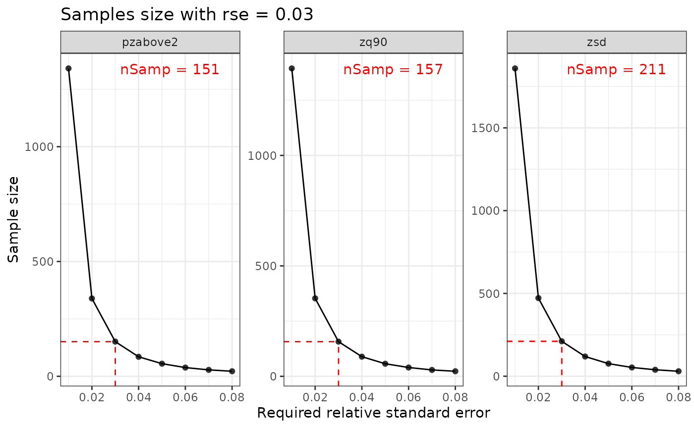
calculate_allocation
calculate_allocation() determines how sample units are
allocated based on the desired sample size (nSamp) and the
input sraster. It is used internally in a number of
algorithms, including sample_strat.
Currently, there are four allocation methods: proportional
(prop; default), optimal (optim), equal
(equal), and manual (manual).
Proportional allocation
Samples are allocated based on the spatial coverage area of the strata. This is the default allocation method.
#--- perform grid sampling ---#
calculate_allocation(
  sraster = sraster,
  nSamp = 200
)
#>   strata total
#> 1      1    51
#> 2      2    50
#> 3      3    49
#> 4      4    50
In this case the sraster has equally sized strata, so the number of allocated sample units is always the same.
#--- calculate existing samples to include ---#
e.sr <- extract_strata(
  sraster = sraster,
  existing = existing
)

calculate_allocation(
  sraster = sraster,
  nSamp = 200,
  existing = e.sr
)
#>   strata total need
#> 1      1     0   51
#> 2      2     0   50
#> 3      3     0   49
#> 4      4     0   50
At times, values under total can be negative. Negative
values indicate that existing sample units over represent
those strata and that some sample units could removed to prevent
over-representation. $total indicates the number of sample
units that could be added or removed.
Optimal Allocation
Sample units are allocated based on within strata variance. The
optimal allocation method uses the variation within the strata metric to
allocate sample units. This means that in addition to providing an
sraster, that a specific metric (mraster) must
be provided to calculate variation to optimally allocate sample
units.
calculate_allocation(
  sraster = sraster, # stratified raster
  nSamp = 200, # desired sample number
  existing = e.sr, # existing samples
  allocation = "optim", # optimal allocation
  mraster = mraster$zq90, # metric raster
  force = TRUE
) # force nSamp number
#> # A tibble: 4 × 3
#> # Rowwise:
#>   strata total  need
#>    <dbl> <dbl> <dbl>
#> 1      1    27    78
#> 2      2   -14    36
#> 3      3   -25    24
#> 4      4    12    62
Equal allocation
There may be situations where the user wants an equal number of
sample units allocated to each strata. In these situations use
allocation = equal. In this case, nSamp refers
to the total number of sample units per strata, instead of the overall
total number.
calculate_allocation(
  sraster = sraster, # stratified raster
  nSamp = 20, # desired sample number
  allocation = "equal"
) # optimal allocation
#> Implementing equal allocation of samples.
#> # A tibble: 4 × 2
#>   strata total
#>    <dbl> <dbl>
#> 1      1    20
#> 2      2    20
#> 3      3    20
#> 4      4    20
The code in the demonstration above yields a total of 80 samples (20
nSamp for each of the 4 strata in
sraster).
Manual allocation
The user may wish to manually assign weights to strata. In this case,
allocation = manual can be used and weights
must be provided as a numeric vector
(e.g. weights = c(0.2, 0.2, 0.2, 0.4) where
sum(weights) == 1). In this case, nSamp will
be allocated based on weights.
weights <- c(0.2, 0.2, 0.2, 0.4)

calculate_allocation(
  sraster = sraster, # stratified raster
  nSamp = 20, # desired sample number
  allocation = "manual", # manual allocation
  weights = weights
) # weights adding to 1
#> Implementing allocation of samples based on user-defined weights.
#>   strata total
#> 1      1     4
#> 2      2     4
#> 3      3     4
#> 4      4     8
The code above yields a total of 20 sample units with plots being
allocated based on the weights provided in ascending strata
order.
Sample evaluation algorithms
The following algorithms were initially developed by Dr. Brendan Malone from the University of Sydney. Dr. Malone and his colleagues supplied an in depth description of the functionality of these algorithms, which were originally developed to improve soil sampling strategies. These functions were modified and implemented to be used for structurally guided sampling approaches. Many thanks to Dr. Malone for being a proponent of open source algorithms.
Please consult the original reference for these scripts and ideas as their publication holds helpful and valuable information to understand their rationale for sampling and algorithm development.
Malone BP, Minansy B, Brungard C. 2019. Some methods to improve the utility of conditioned Latin hypercube sampling. PeerJ 7:e6451 DOI 10.7717/peerj.6451
calculate_coobs
calculate_coobs() function performs the
COunt of OBServations (coobs)
algorithm using an existing sample and
mraster. This algorithm helps the user understand how an
existing sample is distributed among the landscape in
relation to mraster data.
TIP!
The output coobs raster can be used to constrain clhs sampling using
the sample_clhs() function to the areas that are
under-represented.
The coobs raster determines how many observations are similar in terms of the covariate space at every pixel, and takes advantage of parallel processing routines.
calculate_coobs(
  mraster = mraster, # input
  existing = existing, # existing samples
  cores = 4, # parallel cores to use
  details = TRUE, # provide details from algorithm output
  plot = TRUE
) # plot
Latin hypercube sampling evaluation algorithms
The following 2 algorithms present the means to maximize the effectiveness of the latin hypercube sampling protocols.
calculate_pop
calculate_pop() calculates population level statistics
of an mraster, including calculating the principal
components, quantile & covariate distributions, and Kullback-Leibler
divergence testing.
The outputs produced from this functions are required to use the
calculate_lhsOpt() function described in the following
section.
TIP!
This algorithm can be pre-emptively used to calculate
matQ and MatCov, two values that are used for
the sample_ahels() function. This will save processing time
during sampling.
#--- by default all statistical data are calculated ---#
calculate_pop(mraster = mraster) # input
The output list contains the following:
$values- Pixel values frommraster$pcaLoad- PCA loadings$matQ- Quantile matrix$matCov- Covariate matrix
#--- statistical analyses can be chosen by setting their parameter to `FALSE` ---#
mat <- calculate_pop(
  mraster = mraster, # input
  nQuant = 10
) # desired number of quantiles

#--- use matrix output within sample ahels algorithm ---#
sample_ahels(
  mraster = mraster, # input
  existing = existing, # existing sample
  nQuant = 10, # number of desired quantiles
  nSamp = 50, # desired sample size
  matCov = mat
) # covariance matrix
calculate_lhsOpt
calculate_lhsOpt() function performs a bootstrapped
latin hypercube sampling approach where population level analysis of
mraster data is performed to determine the optimal latin
hypercube sample size.
calculate_pop() and varying sample sizes defined by
minSamp, maxSamp, step and
rep. Sampling protocols are conducted and statistical
effectiveness of those sampling outcomes are evaluated to determine
where sample size is minimized and statistical representation is
maximized.
#--- calculate lhsPop details ---#
poplhs <- calculate_pop(mraster = mr)

calculate_lhsOpt(popLHS = poplhs)
calculate_lhsOpt(
  popLHS = poplhs,
  PCA = FALSE,
  iter = 200
)