sgsR

Algorithm structure

sgsR is scripted using the terra package to handle raster processing, and sf package for vector manipulation.

Four primary function verbs exist:

strat_*

Stratification algorithms within sgsR. These algorithms use auxiliary raster data (e.g. ALS metric populations) as inputs and provide stratified areas of interest as outputs. Algorithms are either supervised (e.g. strat_breaks()), where the user provides quantitative values that drive stratifications, or unsupervised (e.g. strat_quantiles()), where the user specifies the desired number of output strata (nStrata) and stratification is handled by the algorithm.

sample_*

Sampling algorithms in sgsR. Depending on the sampling algorithm, users are able to provide either auxiliary metrics or stratifications derived from strat_* functions as inputs. A number of customizable parameters can be set including the sample size (nSamp), a minimum distance threshold (mindist) between allocated sample units, and the ability for the user to define an access network (access) and assign minimum (buff_inner) and maximum (buff_outer) buffer distances to constrain sampling extents.

calculate_* & extract_*

Additional helper functions that calculate varying descriptive / summary statistics and values to use in processing. extract_* functions derive metric values from co-located sample units.

Parameters

sgsR uses common words that define algorithm parameters:

Parameter	Description
mraster	Metric raster(s)
sraster	Stratified raster
access	Linear vectors representing access routes
existing	Existing sample units
plot	Visually displays raster and samples

mraster

mraster are input raster(s). All raster data used by sgsR must be must be a terra SpatRaster class.

library(sgsR)
library(terra)
library(sf)

#--- Load mraster from internal data ---#
r <- system.file("extdata", "mraster.tif", package = "sgsR")

#--- load mraster using the terra package ---#
mraster <- terra::rast(r)

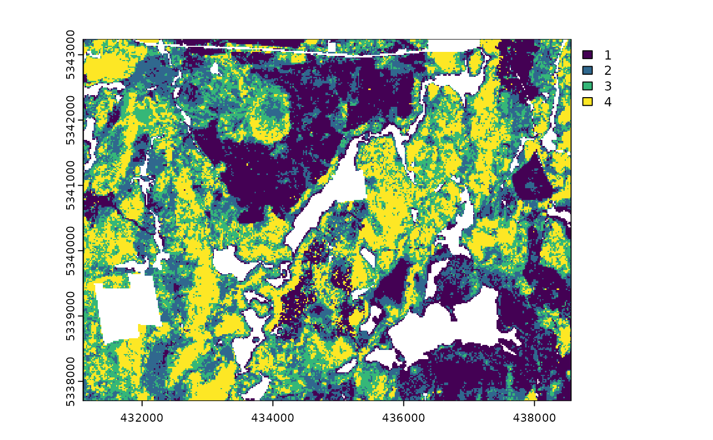
sraster

sraster are derived from strat_* algorithms (e.g. see strat_quantiles() below). The function below used the distribution of mraster$zq90 and stratified data into 4 equally sized strata.

#--- apply kmeans algorithm to metrics raster ---#
sraster <- strat_quantiles(
  mraster = mraster$zq90, # use mraster as input for sampling
  nStrata = 4, # algorithm will produce 4 strata
  plot = TRUE
) # algorithm will plot output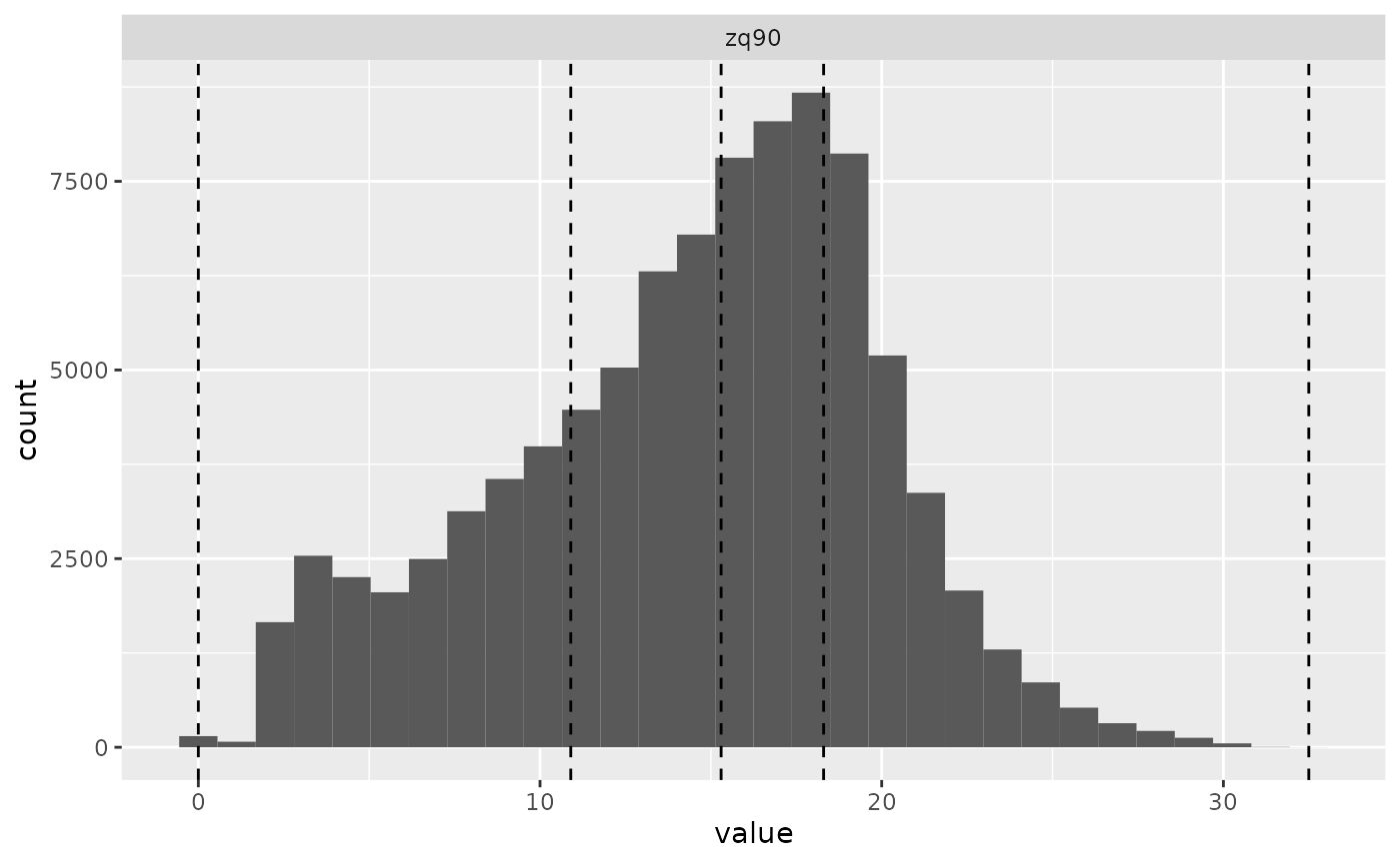

The sraster output can then become an input parameter (sraster) for the sample_strat() algorithm.

#--- apply stratified sampling ---#
existing <- sample_strat(
  sraster = sraster, # use mraster as input for sampling
  nSamp = 200, # request 200 samples be taken
  mindist = 100, # define that samples must be 100 m apart
  plot = TRUE
) # algorithm will plot output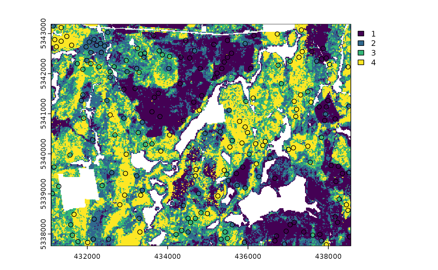

access

One key feature of using some sample_* functions is its ability to define access corridors. Users can supply a road access network (must be sf line objects) and define buffers around access where samples should be excluded and included.

Relevant and applicable parameters when access is defined are:

• buff_inner - Can be left as NULL (default). Inner buffer parameter that defines the distance from access where samples cannot be taken (i.e. if you don’t want samples within 50 m of your access layer set buff_inner = 50).

• buff_outer - Outer buffer parameter that defines the maximum distance that the samples can be located from access (i.e. if you don’t want samples more than 200 meters from your access layer set buff_inner = 200).

a <- system.file("extdata", "access.shp", package = "sgsR")

#--- load the access vector using the sf package ---#
access <- sf::st_read(a)
#> Reading layer `access' from data source 
#>   `/home/runner/work/_temp/Library/sgsR/extdata/access.shp' 
#>   using driver `ESRI Shapefile'
#> Simple feature collection with 167 features and 2 fields
#> Geometry type: MULTILINESTRING
#> Dimension:     XY
#> Bounding box:  xmin: 431100 ymin: 5337700 xmax: 438560 ymax: 5343240
#> Projected CRS: UTM_Zone_17_Northern_Hemisphere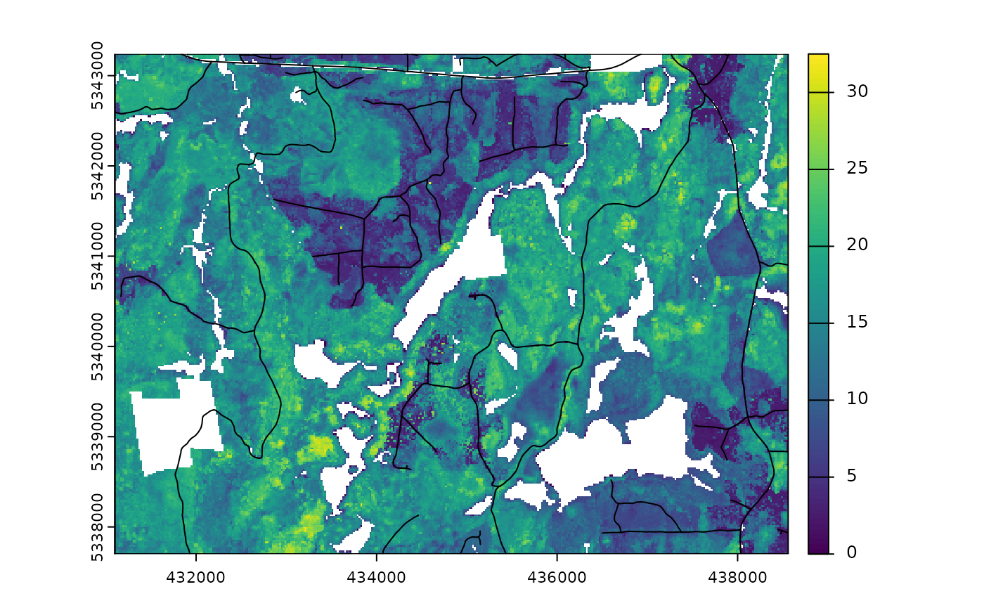

terra::plot(mraster$zq90)
terra::plot(access, add = TRUE, col = "black")

From the plot output we see the first band (zq90) of the mraster with the access vector overlaid.

%>%

The sgsR package leverages the %>% operator from the magrittr package.

#--- non piped ---#
sraster <- strat_quantiles(
  mraster = mraster$zq90, # use mraster as input for sampling
  nStrata = 4
) # algorithm will produce 4 strata

existing <- sample_strat(
  sraster = sraster, # use mraster as input for sampling
  nSamp = 200, # request 200 samples be taken
  mindist = 100
) # define that samples must be 100 m apart

extract_metrics(
  mraster = mraster,
  existing = existing
)

#--- piped ---#
strat_quantiles(mraster = mraster$zq90, nStrata = 4) %>%
  sample_strat(., nSamp = 200, mindist = 100) %>%
  extract_metrics(mraster = mraster, existing = .)