LAScatalog
Relevant resources:
Overview
This code performs various operations on LiDAR data using LAScatalog functionality. We visualize and inspect the data, validate the files, clip the data based on specific coordinates, generate a Canopy Height Model (CHM), compute above ground biomass, detect treetops, specify processing options, and use parallel computing.
Environment
# Clear environment
rm(list = ls(globalenv()))

# Load packages
library(lidR)
library(sf)
Basic Usage
In this section, we will cover the basic usage of the lidR package, including reading LiDAR data, visualization, and inspecting metadata.
Read catalog from directory of files
We begin by creating a LAS catalog (ctg) from a folder containing multiple LAS files using the readLAScatalog() function.
# Read catalog and drop withheld
ctg <- readLAScatalog(folder = "data/Farm_A/",filter = "-drop_withheld")
Inspect catalog
We can inspect the contents of the catalog using standard R functions.
ctg
#> class       : LAScatalog (v1.2 format 0)
#> extent      : 207340, 208040, 7357280, 7357980 (xmin, xmax, ymin, ymax)
#> coord. ref. : SIRGAS 2000 / UTM zone 23S
#> area        : 489930 m²
#> points      : 14.49 million points
#> density     : 29.6 points/m²
#> density     : 23.2 pulses/m²
#> num. files  : 25
Visualize catalog
We visualize the catalog, showing the spatial coverage of the LiDAR data header extents. The map can be interactive if we use map = TRUE. Try clicking on a tile to see its header information.
plot(ctg)
# Interactive
plot(ctg, map = TRUE)
Check coordinate system and extent info
We examine the coordinate system and extent information of the catalog.
# coordinate system
crs(ctg)
#> Coordinate Reference System:
#> Deprecated Proj.4 representation:
#>  +proj=utm +zone=23 +south +ellps=GRS80 +towgs84=0,0,0,0,0,0,0 +units=m
#> +no_defs
#> WKT2 2019 representation:
#> PROJCRS["SIRGAS 2000 / UTM zone 23S",
#>     BASEGEOGCRS["SIRGAS 2000",
#>         DATUM["Sistema de Referencia Geocentrico para las AmericaS 2000",
#>             ELLIPSOID["GRS 1980",6378137,298.257222101,
#>                 LENGTHUNIT["metre",1]]],
#>         PRIMEM["Greenwich",0,
#>             ANGLEUNIT["degree",0.0174532925199433]],
#>         ID["EPSG",4674]],
#>     CONVERSION["UTM zone 23S",
#>         METHOD["Transverse Mercator",
#>             ID["EPSG",9807]],
#>         PARAMETER["Latitude of natural origin",0,
#>             ANGLEUNIT["degree",0.0174532925199433],
#>             ID["EPSG",8801]],
#>         PARAMETER["Longitude of natural origin",-45,
#>             ANGLEUNIT["degree",0.0174532925199433],
#>             ID["EPSG",8802]],
#>         PARAMETER["Scale factor at natural origin",0.9996,
#>             SCALEUNIT["unity",1],
#>             ID["EPSG",8805]],
#>         PARAMETER["False easting",500000,
#>             LENGTHUNIT["metre",1],
#>             ID["EPSG",8806]],
#>         PARAMETER["False northing",10000000,
#>             LENGTHUNIT["metre",1],
#>             ID["EPSG",8807]]],
#>     CS[Cartesian,2],
#>         AXIS["(E)",east,
#>             ORDER[1],
#>             LENGTHUNIT["metre",1]],
#>         AXIS["(N)",north,
#>             ORDER[2],
#>             LENGTHUNIT["metre",1]],
#>     USAGE[
#>         SCOPE["Engineering survey, topographic mapping."],
#>         AREA["Brazil - between 48°W and 42°W, northern and southern hemispheres, onshore and offshore."],
#>         BBOX[-33.5,-48,5.13,-42]],
#>     ID["EPSG",31983]]
projection(ctg)
#> [1] "+proj=utm +zone=23 +south +ellps=GRS80 +towgs84=0,0,0,0,0,0,0 +units=m +no_defs"
st_crs(ctg)
#> Coordinate Reference System:
#>   User input: EPSG:31983
#>   wkt:
#> PROJCRS["SIRGAS 2000 / UTM zone 23S",
#>     BASEGEOGCRS["SIRGAS 2000",
#>         DATUM["Sistema de Referencia Geocentrico para las AmericaS 2000",
#>             ELLIPSOID["GRS 1980",6378137,298.257222101,
#>                 LENGTHUNIT["metre",1]]],
#>         PRIMEM["Greenwich",0,
#>             ANGLEUNIT["degree",0.0174532925199433]],
#>         ID["EPSG",4674]],
#>     CONVERSION["UTM zone 23S",
#>         METHOD["Transverse Mercator",
#>             ID["EPSG",9807]],
#>         PARAMETER["Latitude of natural origin",0,
#>             ANGLEUNIT["degree",0.0174532925199433],
#>             ID["EPSG",8801]],
#>         PARAMETER["Longitude of natural origin",-45,
#>             ANGLEUNIT["degree",0.0174532925199433],
#>             ID["EPSG",8802]],
#>         PARAMETER["Scale factor at natural origin",0.9996,
#>             SCALEUNIT["unity",1],
#>             ID["EPSG",8805]],
#>         PARAMETER["False easting",500000,
#>             LENGTHUNIT["metre",1],
#>             ID["EPSG",8806]],
#>         PARAMETER["False northing",10000000,
#>             LENGTHUNIT["metre",1],
#>             ID["EPSG",8807]]],
#>     CS[Cartesian,2],
#>         AXIS["(E)",east,
#>             ORDER[1],
#>             LENGTHUNIT["metre",1]],
#>         AXIS["(N)",north,
#>             ORDER[2],
#>             LENGTHUNIT["metre",1]],
#>     USAGE[
#>         SCOPE["Engineering survey, topographic mapping."],
#>         AREA["Brazil - between 48°W and 42°W, northern and southern hemispheres, onshore and offshore."],
#>         BBOX[-33.5,-48,5.13,-42]],
#>     ID["EPSG",31983]]

# spatial extents
extent(ctg)
#> class      : Extent
#> xmin       : 207340
#> xmax       : 208040
#> ymin       : 7357280
#> ymax       : 7357980
bbox(ctg)
#>         [,1]    [,2]
#> [1,]  207340  208040
#> [2,] 7357280 7357980
st_bbox(ctg)
#>    xmin    ymin    xmax    ymax
#>  207340 7357280  208040 7357980
Validate files in catalog
We validate the LAS files within the catalog using the las_check function. It works the same way as it would on a regular LAS file.
# Perform a check on the catalog
las_check(las = ctg)
#>
#>  Checking headers consistency
#>   - Checking file version consistency... ✓
#>   - Checking scale consistency... ✓
#>   - Checking offset consistency... ✓
#>   - Checking point type consistency... ✓
#>   - Checking VLR consistency... ✓
#>   - Checking CRS consistency... ✓
#>  Checking the headers
#>   - Checking scale factor validity... ✓
#>   - Checking Point Data Format ID validity... ✓
#>  Checking preprocessing already done
#>   - Checking negative outliers...
#>     ⚠ 25 file(s) with points below 0
#>   - Checking normalization... no
#>  Checking the geometry
#>   - Checking overlapping tiles... ✓
#>   - Checking point indexation... no
File indexing
We explore indexing of LAScatalog objects for efficient processing.
The lidR policy has always been: use LAStools and lasindex for spatial indexing. If you really don’t want, or can’t use LAStools, then there is a hidden function in lidR that users can use (lidR:::catalog_laxindex()).
# check if files have .lax
is.indexed(ctg)
#> [1] FALSE

# generate index files
lidR:::catalog_laxindex(ctg)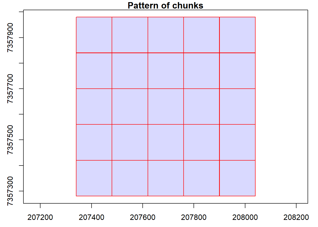
#> Chunk 1 of 25 (4%): state ✓
#> Chunk 2 of 25 (8%): state ✓
#> Chunk 3 of 25 (12%): state ✓
#> Chunk 4 of 25 (16%): state ✓
#> Chunk 5 of 25 (20%): state ✓
#> Chunk 6 of 25 (24%): state ✓
#> Chunk 7 of 25 (28%): state ✓
#> Chunk 8 of 25 (32%): state ✓
#> Chunk 9 of 25 (36%): state ✓
#> Chunk 10 of 25 (40%): state ✓
#> Chunk 11 of 25 (44%): state ✓
#> Chunk 12 of 25 (48%): state ✓
#> Chunk 13 of 25 (52%): state ✓
#> Chunk 14 of 25 (56%): state ✓
#> Chunk 15 of 25 (60%): state ✓
#> Chunk 16 of 25 (64%): state ✓
#> Chunk 17 of 25 (68%): state ✓
#> Chunk 18 of 25 (72%): state ✓
#> Chunk 19 of 25 (76%): state ✓
#> Chunk 20 of 25 (80%): state ✓
#> Chunk 21 of 25 (84%): state ✓
#> Chunk 22 of 25 (88%): state ✓
#> Chunk 23 of 25 (92%): state ✓
#> Chunk 24 of 25 (96%): state ✓
#> Chunk 25 of 25 (100%): state ✓

# check if files have .lax
is.indexed(ctg)
#> [1] TRUE
Generate CHM
We create a CHM by rasterizing the point cloud data from the catalog.
# Generate CHM
chm <- rasterize_canopy(las = ctg, res = 0.5, algorithm = p2r(subcircle = 0.15))
#> Chunk 1 of 25 (4%): state ✓
#> Chunk 2 of 25 (8%): state ✓
#> Chunk 3 of 25 (12%): state ✓
#> Chunk 4 of 25 (16%): state ✓
#> Chunk 5 of 25 (20%): state ✓
#> Chunk 6 of 25 (24%): state ✓
#> Chunk 7 of 25 (28%): state ✓
#> Chunk 8 of 25 (32%): state ✓
#> Chunk 9 of 25 (36%): state ✓
#> Chunk 10 of 25 (40%): state ✓
#> Chunk 11 of 25 (44%): state ✓
#> Chunk 12 of 25 (48%): state ✓
#> Chunk 13 of 25 (52%): state ✓
#> Chunk 14 of 25 (56%): state ✓
#> Chunk 15 of 25 (60%): state ✓
#> Chunk 16 of 25 (64%): state ✓
#> Chunk 17 of 25 (68%): state ✓
#> Chunk 18 of 25 (72%): state ✓
#> Chunk 19 of 25 (76%): state ✓
#> Chunk 20 of 25 (80%): state ✓
#> Chunk 21 of 25 (84%): state ✓
#> Chunk 22 of 25 (88%): state ✓
#> Chunk 23 of 25 (92%): state ✓
#> Chunk 24 of 25 (96%): state ✓
#> Chunk 25 of 25 (100%): state ✓
plot(chm, col = height.colors(50))
We encounter issues and warnings while generating the CHM. Let’s figure out how to fix the warnings and get decent outputs.
# Check for warnings
warnings()
Catalog processing options
We explore and manipulate catalog options.
# Setting options and re-rasterizing the CHM
opt_filter(ctg) <- "-drop_z_below 0 -drop_z_above 40"
opt_select(ctg) <- "xyz"
chm <- rasterize_canopy(las = ctg, res = 0.5, algorithm = p2r(subcircle = 0.15))
#> Chunk 1 of 25 (4%): state ⚠
#> Chunk 2 of 25 (8%): state ⚠
#> Chunk 3 of 25 (12%): state ⚠
#> Chunk 4 of 25 (16%): state ⚠
#> Chunk 5 of 25 (20%): state ⚠
#> Chunk 6 of 25 (24%): state ⚠
#> Chunk 7 of 25 (28%): state ⚠
#> Chunk 8 of 25 (32%): state ⚠
#> Chunk 9 of 25 (36%): state ⚠
#> Chunk 10 of 25 (40%): state ⚠
#> Chunk 11 of 25 (44%): state ⚠
#> Chunk 12 of 25 (48%): state ⚠
#> Chunk 13 of 25 (52%): state ⚠
#> Chunk 14 of 25 (56%): state ⚠
#> Chunk 15 of 25 (60%): state ⚠
#> Chunk 16 of 25 (64%): state ⚠
#> Chunk 17 of 25 (68%): state ⚠
#> Chunk 18 of 25 (72%): state ⚠
#> Chunk 19 of 25 (76%): state ⚠
#> Chunk 20 of 25 (80%): state ⚠
#> Chunk 21 of 25 (84%): state ⚠
#> Chunk 22 of 25 (88%): state ⚠
#> Chunk 23 of 25 (92%): state ⚠
#> Chunk 24 of 25 (96%): state ⚠
#> Chunk 25 of 25 (100%): state ⚠
plot(chm, col = height.colors(50))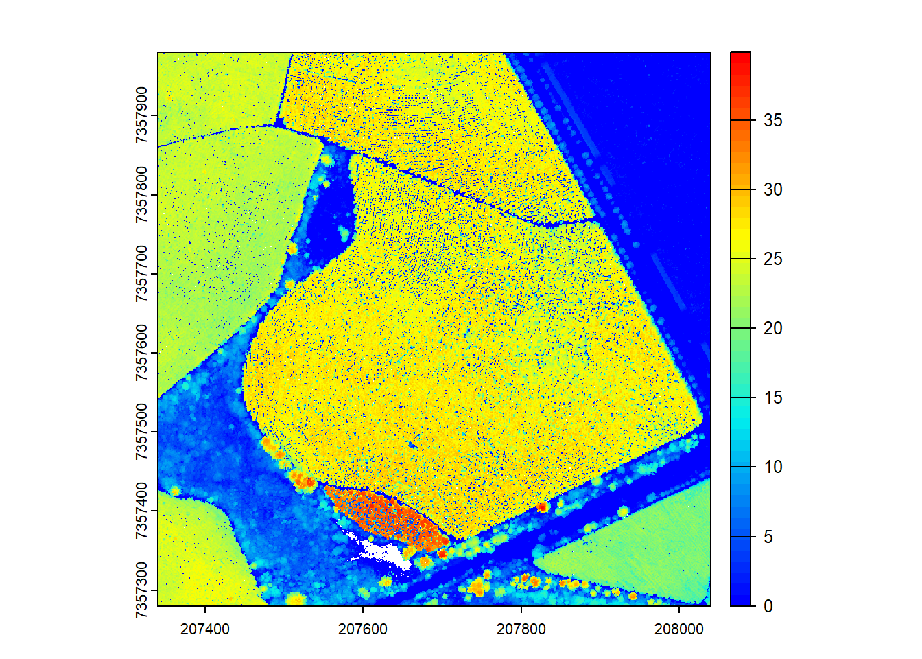
Area-based approach on catalog
In this section, we generate Above Ground Biomass (ABA) estimates using the LAScatalog.
Generate ABA output and visualize
We calculate ABA using the pixel_metrics function and visualize the results.
# Generate area-based metrics
model <- pixel_metrics(las = ctg, func = ~max(Z), res = 20)
#> Chunk 1 of 25 (4%): state ⚠
#> Chunk 2 of 25 (8%): state ⚠
#> Chunk 3 of 25 (12%): state ⚠
#> Chunk 4 of 25 (16%): state ⚠
#> Chunk 5 of 25 (20%): state ⚠
#> Chunk 6 of 25 (24%): state ⚠
#> Chunk 7 of 25 (28%): state ⚠
#> Chunk 8 of 25 (32%): state ⚠
#> Chunk 9 of 25 (36%): state ⚠
#> Chunk 10 of 25 (40%): state ⚠
#> Chunk 11 of 25 (44%): state ⚠
#> Chunk 12 of 25 (48%): state ⚠
#> Chunk 13 of 25 (52%): state ⚠
#> Chunk 14 of 25 (56%): state ⚠
#> Chunk 15 of 25 (60%): state ⚠
#> Chunk 16 of 25 (64%): state ⚠
#> Chunk 17 of 25 (68%): state ⚠
#> Chunk 18 of 25 (72%): state ⚠
#> Chunk 19 of 25 (76%): state ⚠
#> Chunk 20 of 25 (80%): state ⚠
#> Chunk 21 of 25 (84%): state ⚠
#> Chunk 22 of 25 (88%): state ⚠
#> Chunk 23 of 25 (92%): state ⚠
#> Chunk 24 of 25 (96%): state ⚠
#> Chunk 25 of 25 (100%): state ⚠
plot(model, col = height.colors(50))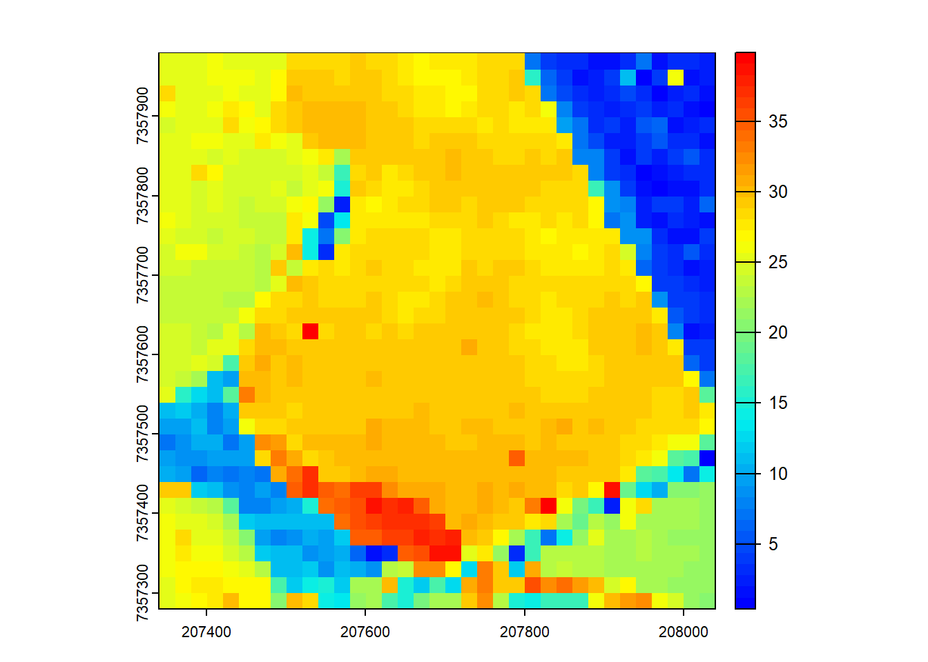
First returns only
We adjust the catalog options to calculate ABA based on first returns only.
opt_filter(ctg) <- "-drop_z_below 0 -drop_z_above 40 -keep_first"
model <- pixel_metrics(las = ctg, func = ~max(Z), res = 20)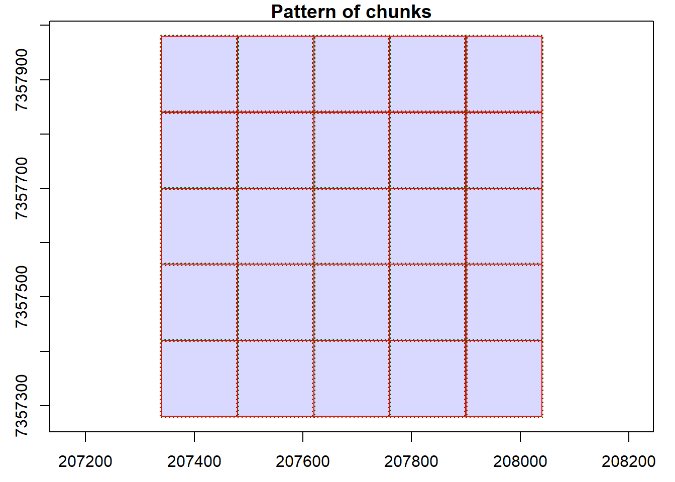
#> Chunk 1 of 25 (4%): state ⚠
#> Chunk 2 of 25 (8%): state ⚠
#> Chunk 3 of 25 (12%): state ⚠
#> Chunk 4 of 25 (16%): state ⚠
#> Chunk 5 of 25 (20%): state ⚠
#> Chunk 6 of 25 (24%): state ⚠
#> Chunk 7 of 25 (28%): state ⚠
#> Chunk 8 of 25 (32%): state ⚠
#> Chunk 9 of 25 (36%): state ⚠
#> Chunk 10 of 25 (40%): state ⚠
#> Chunk 11 of 25 (44%): state ⚠
#> Chunk 12 of 25 (48%): state ⚠
#> Chunk 13 of 25 (52%): state ⚠
#> Chunk 14 of 25 (56%): state ⚠
#> Chunk 15 of 25 (60%): state ⚠
#> Chunk 16 of 25 (64%): state ⚠
#> Chunk 17 of 25 (68%): state ⚠
#> Chunk 18 of 25 (72%): state ⚠
#> Chunk 19 of 25 (76%): state ⚠
#> Chunk 20 of 25 (80%): state ⚠
#> Chunk 21 of 25 (84%): state ⚠
#> Chunk 22 of 25 (88%): state ⚠
#> Chunk 23 of 25 (92%): state ⚠
#> Chunk 24 of 25 (96%): state ⚠
#> Chunk 25 of 25 (100%): state ⚠
plot(model, col = height.colors(50))
Clip a catalog
We clip the LAS data in the catalog using specified coordinate groups.
# Set coordinate groups
x <- c(207846, 208131, 208010, 207852, 207400)
y <- c(7357315, 7357537, 7357372, 7357548, 7357900)

# Visualize coordinate groups
plot(ctg)
points(x, y)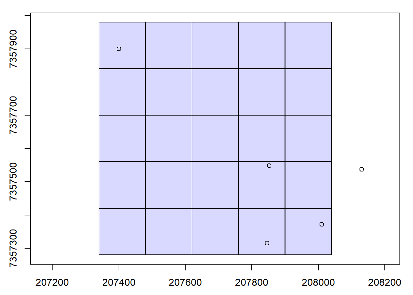
# Clip plots
rois <- clip_circle(las = ctg, xcenter = x, ycenter = y, radius = 30)
#> Chunk 1 of 5 (20%): state ✓
#> Chunk 2 of 5 (40%): state ∅
#> Chunk 3 of 5 (60%): state ✓
#> Chunk 4 of 5 (80%): state ✓
#> Chunk 5 of 5 (100%): state ✓plot(rois[[1]])
plot(rois[[3]])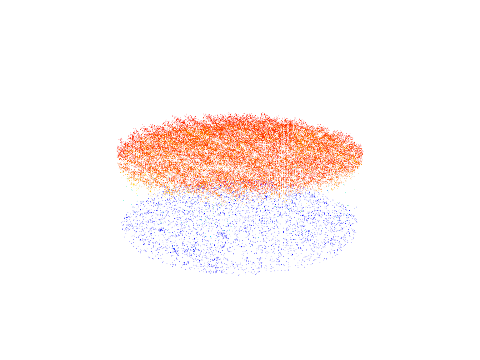
Validate clipped data
We validate the clipped LAS data using the las_check function.
las_check(rois[[1]])
#>
#>  Checking the data
#>   - Checking coordinates... ✓
#>   - Checking coordinates type... ✓
#>   - Checking coordinates range... ✓
#>   - Checking coordinates quantization... ✓
#>   - Checking attributes type... ✓
#>   - Checking ReturnNumber validity... ✓
#>   - Checking NumberOfReturns validity... ✓
#>   - Checking ReturnNumber vs. NumberOfReturns... ✓
#>   - Checking RGB validity... ✓
#>   - Checking absence of NAs... ✓
#>   - Checking duplicated points...
#>     ⚠ 10212 points are duplicated and share XYZ coordinates with other points
#>   - Checking degenerated ground points... skipped
#>   - Checking attribute population... ✓
#>   - Checking gpstime incoherances skipped
#>   - Checking flag attributes... ✓
#>   - Checking user data attribute... skipped
#>  Checking the header
#>   - Checking header completeness... ✓
#>   - Checking scale factor validity... ✓
#>   - Checking point data format ID validity... ✓
#>   - Checking extra bytes attributes validity... ✓
#>   - Checking the bounding box validity... ✓
#>   - Checking coordinate reference system... ✓
#>  Checking header vs data adequacy
#>   - Checking attributes vs. point format... ✓
#>   - Checking header bbox vs. actual content... ✓
#>   - Checking header number of points vs. actual content... ✓
#>   - Checking header return number vs. actual content... ✓
#>  Checking coordinate reference system...
#>   - Checking if the CRS was understood by R... ✓
#>  Checking preprocessing already done
#>   - Checking ground classification... skipped
#>   - Checking normalization... yes
#>   - Checking negative outliers... ✓
#>   - Checking flightline classification... skipped
#>  Checking compression
#>   - Checking attribute compression... no
las_check(rois[[3]])
#>
#>  Checking the data
#>   - Checking coordinates... ✓
#>   - Checking coordinates type... ✓
#>   - Checking coordinates range... ✓
#>   - Checking coordinates quantization... ✓
#>   - Checking attributes type... ✓
#>   - Checking ReturnNumber validity... ✓
#>   - Checking NumberOfReturns validity... ✓
#>   - Checking ReturnNumber vs. NumberOfReturns... ✓
#>   - Checking RGB validity... ✓
#>   - Checking absence of NAs... ✓
#>   - Checking duplicated points...
#>     ⚠ 30645 points are duplicated and share XYZ coordinates with other points
#>   - Checking degenerated ground points... skipped
#>   - Checking attribute population... ✓
#>   - Checking gpstime incoherances skipped
#>   - Checking flag attributes... ✓
#>   - Checking user data attribute... skipped
#>  Checking the header
#>   - Checking header completeness... ✓
#>   - Checking scale factor validity... ✓
#>   - Checking point data format ID validity... ✓
#>   - Checking extra bytes attributes validity... ✓
#>   - Checking the bounding box validity... ✓
#>   - Checking coordinate reference system... ✓
#>  Checking header vs data adequacy
#>   - Checking attributes vs. point format... ✓
#>   - Checking header bbox vs. actual content... ✓
#>   - Checking header number of points vs. actual content... ✓
#>   - Checking header return number vs. actual content... ✓
#>  Checking coordinate reference system...
#>   - Checking if the CRS was understood by R... ✓
#>  Checking preprocessing already done
#>   - Checking ground classification... skipped
#>   - Checking normalization... no
#>   - Checking negative outliers... ✓
#>   - Checking flightline classification... skipped
#>  Checking compression
#>   - Checking attribute compression... no
Independent files (e.g. plots) as catalogs
We read an individual LAS file as a catalog and perform operations on it.
# Read single file as catalog
ctg_non_norm <- readLAScatalog(folder = "data/MixedEucaNat.laz")

# Set options for output files
opt_output_files(ctg_non_norm) <- paste0(tempdir(),"/{XCENTER}_{XCENTER}")

# Write file as .laz
opt_laz_compression(ctg_non_norm) <- TRUE

# Get random plot locations and clip
x <- runif(n = 4, min = ctg_non_norm$Min.X, max = ctg_non_norm$Max.X)
y <- runif(n = 4, min = ctg_non_norm$Min.Y, max = ctg_non_norm$Max.Y)
rois <- clip_circle(las = ctg_non_norm, xcenter = x, ycenter = y, radius = 10)
#> Chunk 1 of 4 (25%): state ✓
#> Chunk 2 of 4 (50%): state ✓
#> Chunk 3 of 4 (75%): state ✓
#> Chunk 4 of 4 (100%): state ✓
# Read catalog of plots
ctg_plots <- readLAScatalog(tempdir())
# Set independent files option
opt_independent_files(ctg_plots) <- TRUE
opt_output_files(ctg_plots) <- paste0(tempdir(),"/{XCENTER}_{XCENTER}")
# Generate plot-level terrain models
rasterize_terrain(las = ctg_plots, res = 1, algorithm = tin())
#> Chunk 1 of 4 (25%): state ✓
#> Chunk 2 of 4 (50%): state ⚠
#> Chunk 3 of 4 (75%): state ✓
#> Chunk 4 of 4 (100%): state ⚠
#> class       : SpatRaster
#> dimensions  : 109, 88, 1  (nrow, ncol, nlyr)
#> resolution  : 1, 1  (x, y)
#> extent      : 203882, 203970, 7358941, 7359050  (xmin, xmax, ymin, ymax)
#> coord. ref. : SIRGAS 2000 / UTM zone 23S (EPSG:31983)
#> source      : rasterize_terrain.vrt
#> name        :      Z
#> min value   : 763.93
#> max value   : 773.49
# Check files
path <- paste0(tempdir())
file_list <- list.files(path, full.names = TRUE)
file <- file_list[grep("\\.tif$", file_list)][[1]]
# plot dtm
plot(terra::rast(file))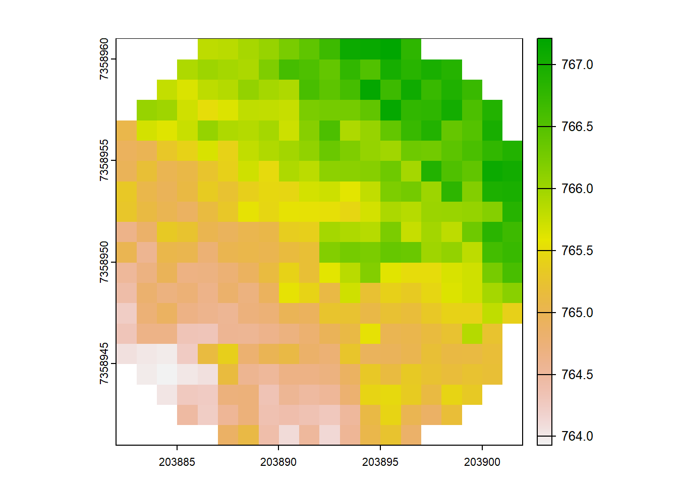
ITD using LAScatalog
In this section, we explore Individual Tree Detection (ITD) using the LAScatalog. We first configure catalog options for ITD.
# Set catalog options
opt_filter(ctg) <- "-drop_withheld -drop_z_below 0 -drop_z_above 40"
Detect treetops and visualize
We detect treetops and visualize the results.
# Detect tree tops and plot
ttops <- locate_trees(las = ctg, algorithm = lmf(ws = 3, hmin = 5))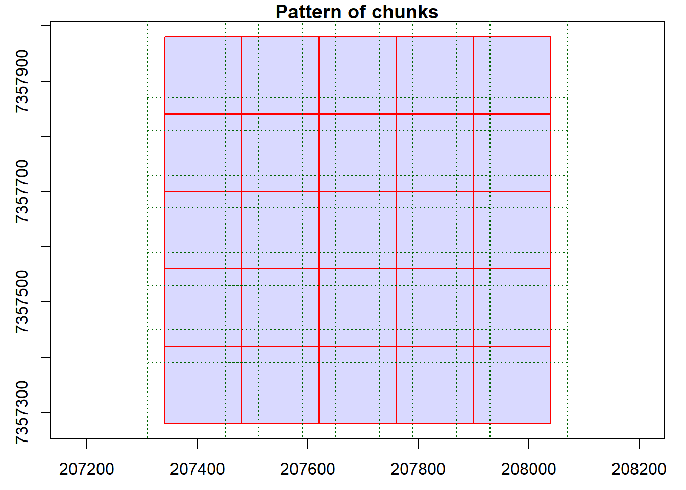
#> Chunk 1 of 25 (4%): state ✓
#> Chunk 2 of 25 (8%): state ✓
#> Chunk 3 of 25 (12%): state ✓
#> Chunk 4 of 25 (16%): state ✓
#> Chunk 5 of 25 (20%): state ✓
#> Chunk 6 of 25 (24%): state ✓
#> Chunk 7 of 25 (28%): state ✓
#> Chunk 8 of 25 (32%): state ✓
#> Chunk 9 of 25 (36%): state ✓
#> Chunk 10 of 25 (40%): state ✓
#> Chunk 11 of 25 (44%): state ✓
#> Chunk 12 of 25 (48%): state ✓
#> Chunk 13 of 25 (52%): state ✓
#> Chunk 14 of 25 (56%): state ✓
#> Chunk 15 of 25 (60%): state ✓
#> Chunk 16 of 25 (64%): state ✓
#> Chunk 17 of 25 (68%): state ✓
#> Chunk 18 of 25 (72%): state ✓
#> Chunk 19 of 25 (76%): state ✓
#> Chunk 20 of 25 (80%): state ✓
#> Chunk 21 of 25 (84%): state ✓
#> Chunk 22 of 25 (88%): state ✓
#> Chunk 23 of 25 (92%): state ✓
#> Chunk 24 of 25 (96%): state ✓
#> Chunk 25 of 25 (100%): state ✓
plot(chm, col = height.colors(50))
plot(ttops, add = TRUE, cex = 0.1, col = "black")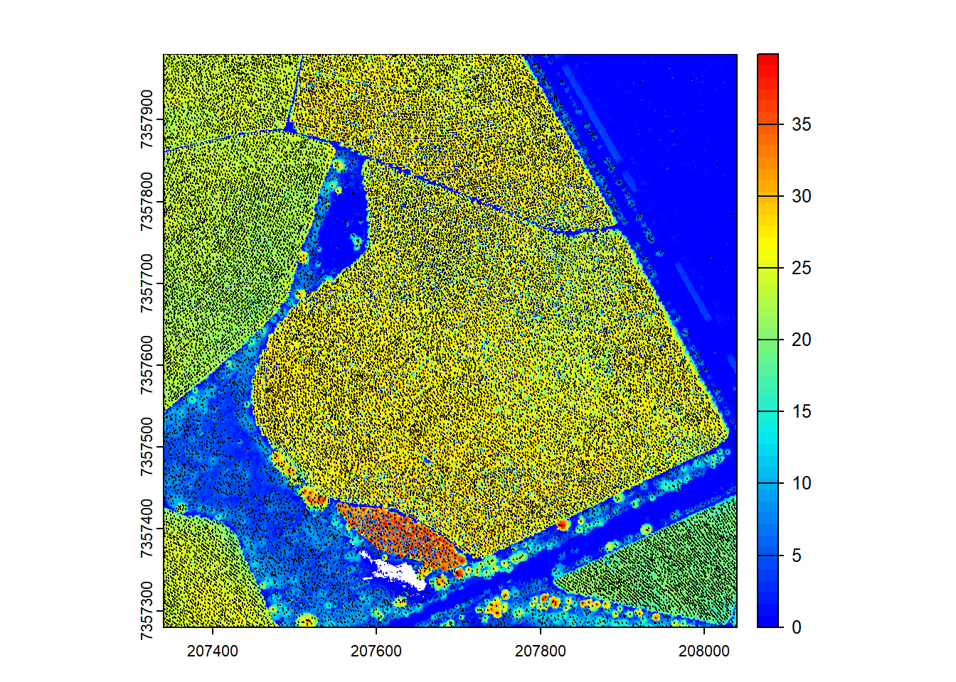
Specify catalog options
We specify additional catalog options for ITD.
# Specify more options
opt_select(ctg) <- "xyz"
opt_chunk_size(ctg) <- 300
opt_chunk_buffer(ctg) <- 10

# Detect treetops and plot
ttops <- locate_trees(las = ctg, algorithm = lmf(ws = 3, hmin = 5))
#> Chunk 1 of 9 (11.1%): state ✓
#> Chunk 2 of 9 (22.2%): state ✓
#> Chunk 3 of 9 (33.3%): state ✓
#> Chunk 4 of 9 (44.4%): state ✓
#> Chunk 5 of 9 (55.6%): state ✓
#> Chunk 6 of 9 (66.7%): state ✓
#> Chunk 7 of 9 (77.8%): state ✓
#> Chunk 8 of 9 (88.9%): state ✓
#> Chunk 9 of 9 (100%): state ✓
plot(chm, col = height.colors(50))
plot(ttops, add = TRUE, cex = 0.1, col = "black")
Parallel computing
In this section, we explore parallel computing using the lidR package.
Load future library
We load the future library to enable parallel processing.
library(future)Specify catalog options
We specify catalog options for parallel processing.
# Specify options
opt_select(ctg) <- "xyz"
opt_chunk_size(ctg) <- 300
opt_chunk_buffer(ctg) <- 10

# Visualize and summarize the catalog chunks
plot(ctg, chunk = TRUE)
summary(ctg)
#> class       : LAScatalog (v1.2 format 0)
#> extent      : 207340, 208040, 7357280, 7357980 (xmin, xmax, ymin, ymax)
#> coord. ref. : SIRGAS 2000 / UTM zone 23S
#> area        : 489930 m²
#> points      : 14.49 million points
#> density     : 29.6 points/m²
#> density     : 23.2 pulses/m²
#> num. files  : 25
#> proc. opt.  : buffer: 10 | chunk: 300
#> input opt.  : select: xyz | filter: -drop_withheld -drop_z_below 0 -drop_z_above 40
#> output opt. : in memory | w2w guaranteed | merging enabled
#> drivers     :
#>  - Raster : format = GTiff  NAflag = -999999
#>  - stars : NA_value = -999999
#>  - SpatRaster : overwrite = FALSE  NAflag = -999999
#>  - SpatVector : overwrite = FALSE
#>  - LAS : no parameter
#>  - Spatial : overwrite = FALSE
#>  - sf : quiet = TRUE
#>  - data.frame : no parameter
Single core processing
We perform tree detection using a single core.
# Process on single core
future::plan(sequential)

# Detect trees
ttops <- locate_trees(las = ctg, algorithm = lmf(ws = 3, hmin = 5))
#> Chunk 1 of 9 (11.1%): state ✓
#> Chunk 2 of 9 (22.2%): state ✓
#> Chunk 3 of 9 (33.3%): state ✓
#> Chunk 4 of 9 (44.4%): state ✓
#> Chunk 5 of 9 (55.6%): state ✓
#> Chunk 6 of 9 (66.7%): state ✓
#> Chunk 7 of 9 (77.8%): state ✓
#> Chunk 8 of 9 (88.9%): state ✓
#> Chunk 9 of 9 (100%): state ✓
Parallel processing
We perform tree detection using multiple cores in parallel.
# Process multi-core
future::plan(multisession)

# Detect trees
ttops <- locate_trees(las = ctg, algorithm = lmf(ws = 3, hmin = 5))
#> Chunk 1 of 9 (11.1%): state ✓
#> Chunk 2 of 9 (22.2%): state ✓
#> Chunk 3 of 9 (33.3%): state ✓
#> Chunk 4 of 9 (44.4%): state ✓
#> Chunk 6 of 9 (55.6%): state ✓
#> Chunk 5 of 9 (66.7%): state ✓
#> Chunk 9 of 9 (77.8%): state ✓
#> Chunk 7 of 9 (88.9%): state ✓
#> Chunk 8 of 9 (100%): state ✓
Revert to single core
We revert to single core processing using future::plan(sequential).
# Back to single core
future::plan(sequential)
This concludes the tutorial on basic usage, catalog validation, indexing, CHM generation, ABA estimation, data clipping, ITD using catalog, and parallel computing using the lidR package in R.
Exercises and Questions
This exercise is complex because it involves options not yet described. Be sure to use the lidRbook and package documentation.
Using:
ctg <- readLAScatalog(folder = "data/Farm_A/")
E1.
Generate a raster of point density for the provided catalog. Hint: Look through the documentation for a function that will do this!
E2.
Modify the catalog to have a point density of 10 pts/m2 using the decimate_points() function. If you get an error make sure to read the documentation for decimate_points() and try: using opt_output_file() to write files to a temporary directory.
E3.
Generate a raster of point density for this new decimated dataset.
E4.
Read the whole decimated catalog as a single las file. The catalog isn’t very big - not recommended for larger datasets!
E5.
Read documentation for the catalog_retile() function and merge the decimated catalog into larger tiles.