Canopy Height Models
Relevant Resources
Overview
This code demonstrates the creation of a Canopy Height Model (CHM). It shows different algorithms for generating CHMs and provides options for adjusting resolution and filling empty pixels.
Environment
# Clear environment
rm(list = ls(globalenv()))

# Load packages
library(lidR)
library(microbenchmark)
library(terra)
Data Preprocessing
We load the LiDAR, keep a random fraction to reduce point density, and visualize the resulting point cloud.
# Load LiDAR data and reduce point density
las <- readLAS(files = "data/MixedEucaNat_normalized.laz", filter = "-keep_random_fraction 0.4 -set_withheld_flag 0")
col <- height.colors(50)
# Visualize the LiDAR point cloud
plot(las)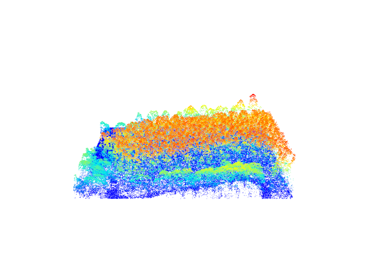
Point-to-Raster Based Algorithm
We demonstrate a simple method for generating Canopy Height Models (CHMs) that assigns the elevation of the highest point to each pixel at a 2 meter spatial resolution.
# Generate the CHM using a simple point-to-raster based algorithm
chm <- rasterize_canopy(las = las, res = 2, algorithm = p2r())

# Visualize the CHM
plot(chm, col = col)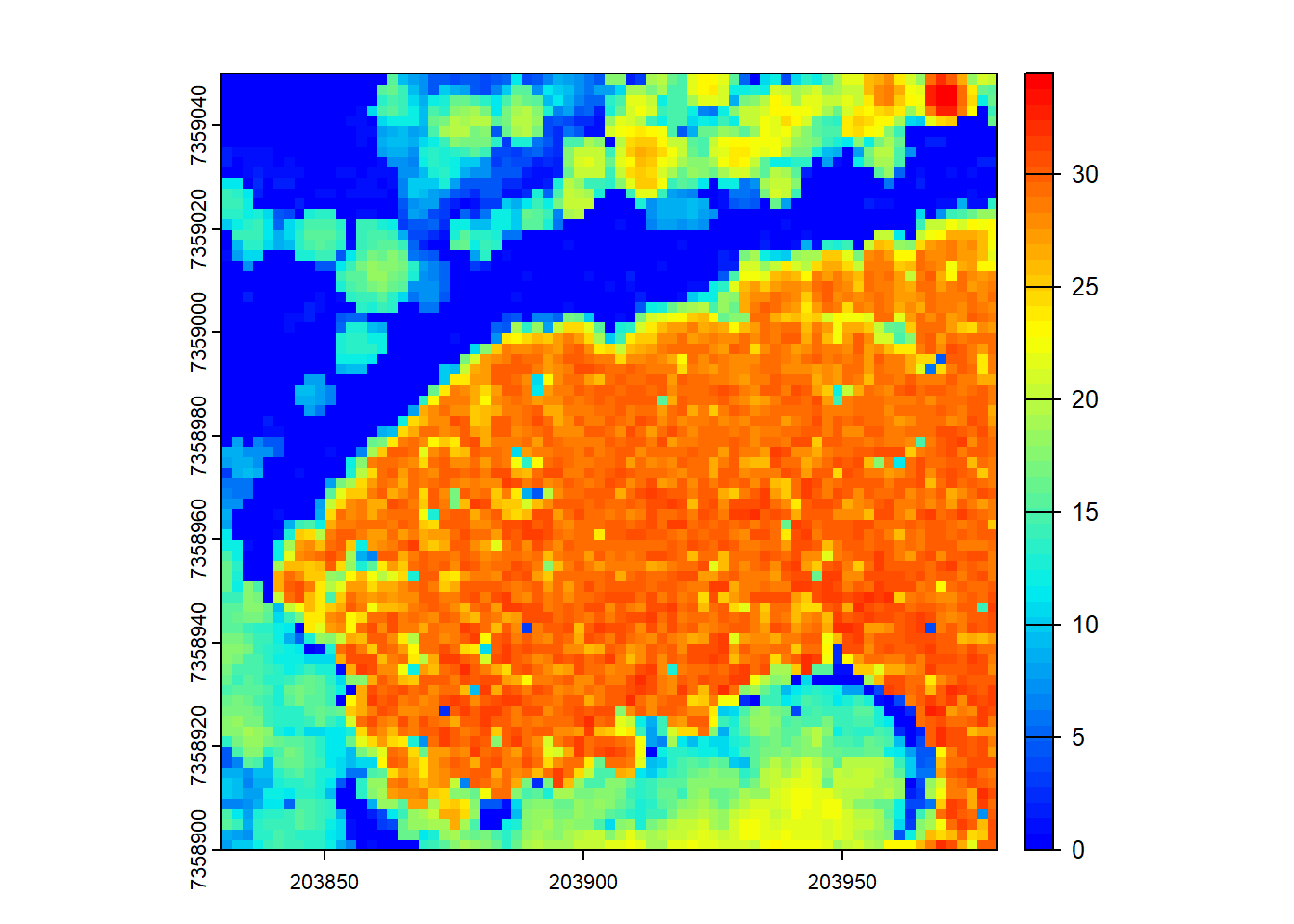
In the first code chunk, we generate a CHM using a point-to-raster based algorithm. The rasterize_canopy() function with the p2r() algorithm assigns the elevation of the highest point within each grid cell to the corresponding pixel. The resulting CHM is then visualized using the plot() function.
# Compute max height using pixel_metrics
chm <- pixel_metrics(las = las, func = ~max(Z), res = 2)

# Visualize the CHM
plot(chm, col = col)
The code chunk above shows that the point-to-raster based algorithm is equivalent to using pixel_metrics with a function that computes the maximum height (max(Z)) within each grid cell. The resulting CHM is visualized using the plot() function.
# However, the rasterize_canopy algorithm is optimized
microbenchmark::microbenchmark(canopy = rasterize_canopy(las = las, res = 1, algorithm = p2r()),
                               metrics = pixel_metrics(las = las, func = ~max(Z), res = 1),
                               times = 10)
#> Unit: milliseconds
#>     expr     min       lq     mean   median       uq      max neval
#>   canopy 43.6846  44.0657  48.4134  45.2242  51.0504  68.5818    10
#>  metrics 98.8050 106.9167 123.8101 115.2184 149.6849 153.4142    10
The above code chunk uses microbenchmark::microbenchmark() to compare the performance of the rasterize_canopy() function with p2r() algorithm and pixel_metrics() function with max(Z) for maximum height computation. It demonstrates that the rasterize_canopy() function is optimized for generating CHMs.
# Make spatial resolution 1 m
chm <- rasterize_canopy(las = las, res = 1, algorithm = p2r())
plot(chm, col = col)
By increasing the resolution of the CHM (reducing the grid cell size), we get a more detailed representation of the canopy, but also have more empty pixels.
# Using the 'subcircle' option turns each point into a disc of 8 points with a radius r
chm <- rasterize_canopy(las = las, res = 0.5, algorithm = p2r(subcircle = 0.15))
plot(chm, col = col)
The rasterize_canopy() function with the p2r() algorithm allows the use of the subcircle option, which turns each LiDAR point into a disc of 8 points with a specified radius. This can help to capture more fine-grained canopy details in the resulting CHM.
# Increasing the subcircle radius, but it may not have meaningful results
chm <- rasterize_canopy(las = las, res = 0.5, algorithm = p2r(subcircle = 0.8))
plot(chm, col = col)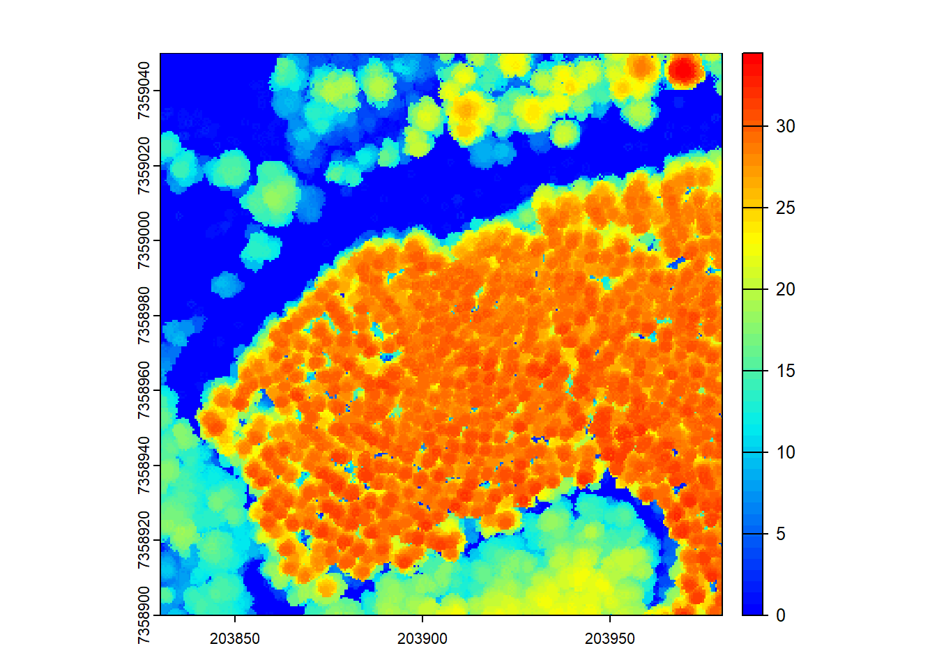
Increasing the subcircle radius may not necessarily result in meaningful CHMs, as it could lead to over-smoothing or loss of important canopy information.
# We can fill empty pixels using TIN interpolation
chm <- rasterize_canopy(las = las, res = 0.5, algorithm = p2r(subcircle = 0.15, na.fill = tin()))
plot(chm, col = col)![]()
The p2r() algorithm also allows filling empty pixels using TIN (Triangulated Irregular Network) interpolation, which can help in areas with sparse LiDAR points to obtain a smoother CHM.
Triangulation Based Algorithm
We demonstrate a triangulation-based algorithm for generating CHMs.
# Triangulation of first returns to generate the CHM
chm <- rasterize_canopy(las = las, res = 1, algorithm = dsmtin())
plot(chm, col = col)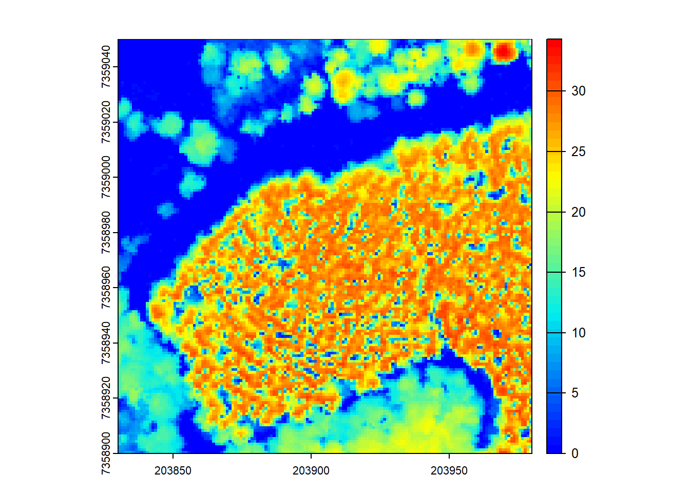
The rasterize_canopy() function with the dsmtin() algorithm generates a CHM by performing triangulation on the first returns from the LiDAR data. The resulting CHM represents the surface of the canopy.
# Increasing the resolution results in a more detailed CHM
chm <- rasterize_canopy(las = las, res = 0.5, algorithm = dsmtin())
plot(chm, col = col)
Increasing the resolution of the CHM using the res argument provides a more detailed representation of the canopy, capturing finer variations in the vegetation.
# Using the Khosravipour et al. 2014 pit-free algorithm with specified thresholds and maximum edge length
thresholds <- c(0, 5, 10, 20, 25, 30)
max_edge <- c(0, 1.35)
chm <- rasterize_canopy(las = las, res = 0.5, algorithm = pitfree(thresholds, max_edge))
plot(chm, col = col)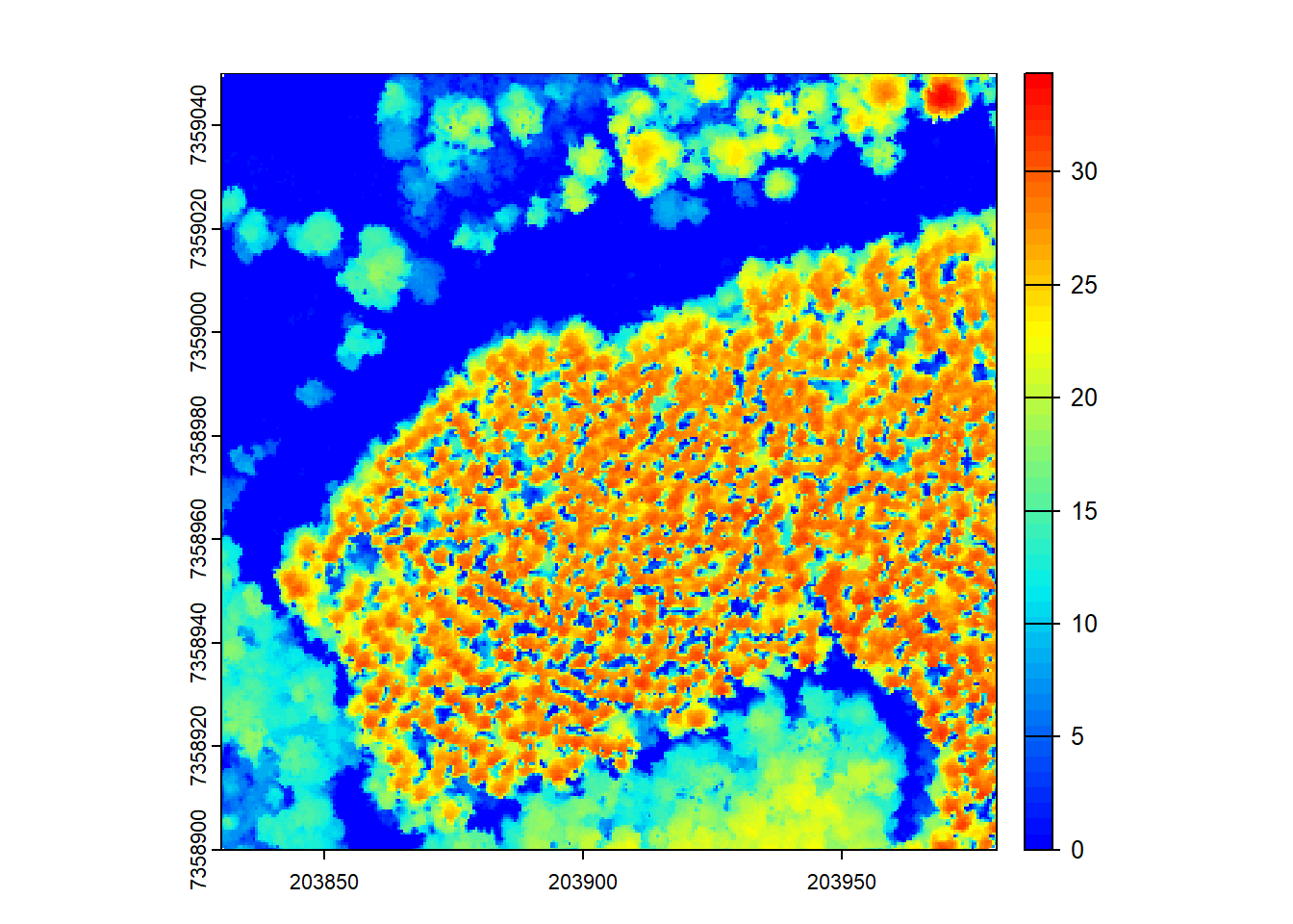
The rasterize_canopy function can also use the Khosravipour et al. 2014 pit-free algorithm with specified height thresholds and a maximum edge length to generate a CHM. This algorithm aims to correct depressions in the CHM surface.
Check out Khosravipour et al. 2014 to see the original implementation of the algorithm!
# Using the 'subcircle' option with the pit-free algorithm
chm <- rasterize_canopy(las = las, res = 0.5, algorithm = pitfree(thresholds, max_edge, 0.1))
plot(chm, col = col)
The subcircle option can be used with the pit-free algorithm to create finer spatial resolution CHMs with subcircles for each LiDAR point, similar to the point-to-raster based algorithm.
Post-Processing
CHMs can be post-processed by smoothing or other manipulations. Here, we demonstrate post-processing using the terra::focal() function for average smoothing within a 3x3 moving window.
# Post-process the CHM using the 'terra' package and focal() function for smoothing
ker <- matrix(1, 3, 3)
schm <- terra::focal(chm, w = ker, fun = mean, na.rm = TRUE)

# Visualize the smoothed CHM
plot(schm, col = col)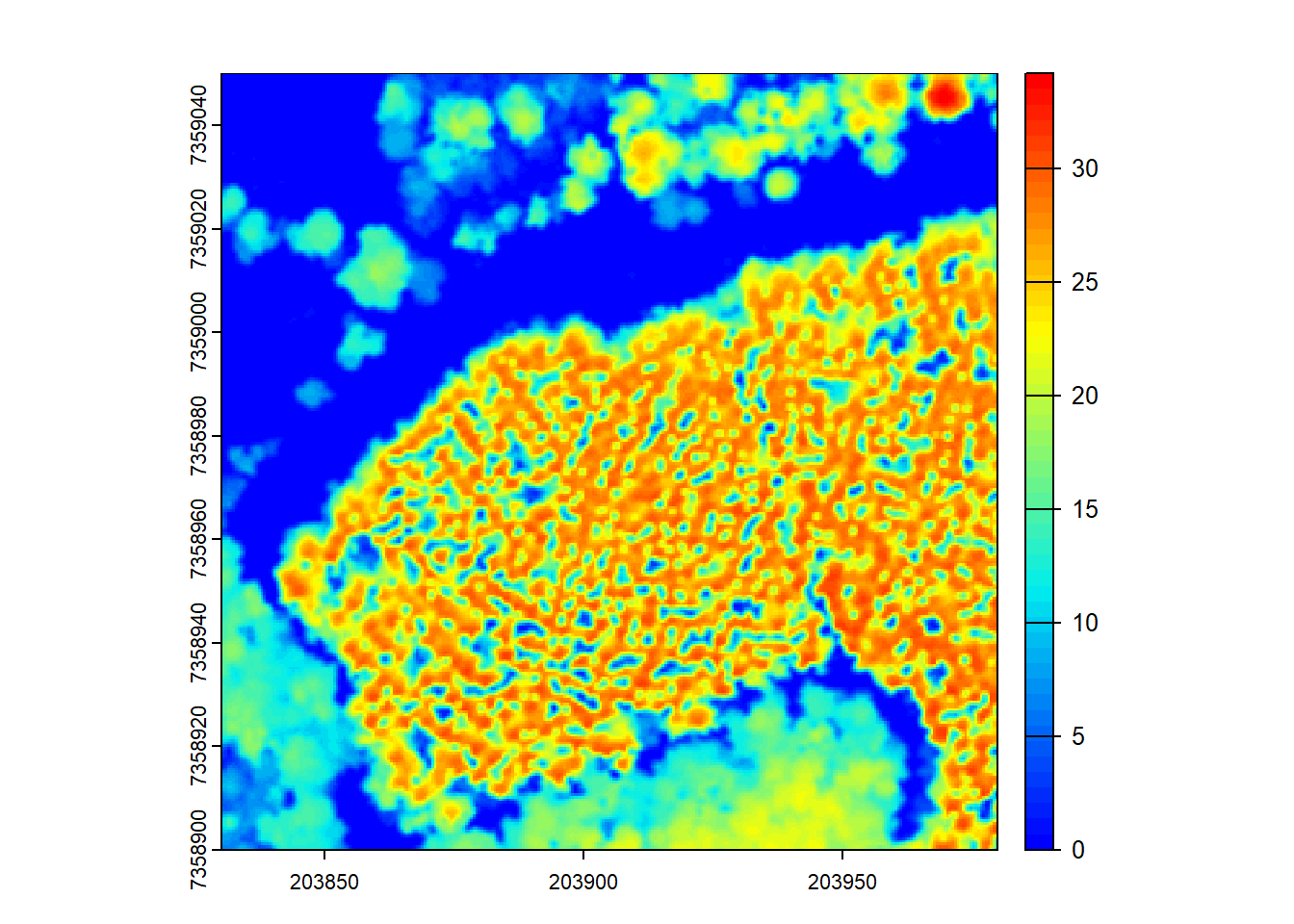
Conclusion
This tutorial covered different algorithms for generating Canopy Height Models (CHMs) from LiDAR data using the lidR package in R. It includes point-to-raster-based algorithms and triangulation-based algorithms, as well as post-processing using the terra package. The code chunks are well-labeled to help the audience navigate through the tutorial easily.